on
A computer scientists' guide to qubits
This is a light introduction to quantum computing and qubits geared towards computer scientists with no background in quantum physics, starting with the very basics: a mathematic view on qubits.
The qubit
The smallest unit in a quantum computer is the qubit, which is used to execute operations, similar to what bits do in a classical computer. You might have heard that the qubits in a quantum computer can be in the states 0 and 1 at the same time, as opposed to classical bits, which can only be in either 0 or 1 at any given time. But how does this actually work on a formal level? Since we’re talking about a quantum computer here, we will need a bit of notation used in quantum mechanics, which is called bra-ket or Dirac notation. This notation is commonly used to describe quantum mechanical states which are represented by vectors. The difference to the common notation used for vectors is that bra-ket vectors are coordinate-free, so one does not have to pick a basis to describe them. Technically we can not write an equals sign between a ket and its corresponding vector, because they are not the same mathematical object, but we will do so here to ease notation. Qubits are just the simplest quantum mechanical states and look like the following in bra-ket notation:
\[\vert 0\rangle = \begin{pmatrix} 1\\ 0 \end{pmatrix}, ~\vert 1\rangle = \begin{pmatrix} 0\\ 1 \end{pmatrix}\]These are called ket, and what hides behind this notation is actually just a column vector of length two. These two vectors form our computational basis states, and we will see later why they are special. Each ket has a corresponding bra (hence the name), which looks as follows for the \(\vert 0 \rangle\) state vector:
\[\langle 0\vert = \vert 0\rangle^*\]The state vectors are elements of the two dimensional complex vector space \(\mathbb{C}^2\). The bra is the transpose of the ket, so it is a row vector. Because the elements of the state vector are complex, we can not simply transpose the ket, but also have to conjugate its elements. In more general terms, our state vectors \(v \in \mathbb{C}^m\) are represented as
\[\vert v\rangle = (v_1, ..., v_m)^T\] \[\langle v\vert = (v_1^*, ..., v_m^*)\]Now you might wonder how a qubit can work its magic if it is only made up of vectors? The computational basis states can be seen as analogues of our classical bit states 0 and 1, so let’s now look at how we can represent a qubit being in a state different from 0 and 1. We now have a quantum mechanical state \(\psi\) that looks as follows:
\[\vert \psi\rangle = \alpha \vert 0\rangle + \beta \vert 1\rangle\]were \(\alpha\) and \(\beta\) are complex numbers called amplitudes, that represent the probability of our qubit being in either state 0 or 1. Remember that probabilities always have to sum up to 1, so we get the additional rule that
\[\vert \alpha\vert ^2 + \vert \beta\vert ^2 = 1\]where we take the absolute square of \(\alpha\) and \(\beta\), because they are complex numbers. So when we say that the qubit is in the states 0 and 1 “at the same time”, we actually mean that \(\alpha\) and \(\beta\) are both non-zero. We then say that the qubit is in a superposition state. The amplitudes now tell us with what probability we will get which computational basis state when we measure the qubit. For example, if we look at the state
\[\vert \psi\rangle = (0.6+0i)\vert 0\rangle + (0.8+0i)\vert 1\rangle\]we would measure a zero with probability \(\vert 0.6 \vert^2 = 0.35\) and a one with probability \(\vert 0.8\vert^2 = 0.65\). This is the catch: the amplitudes can be arbitrarily set between both basis states (as long as their squares sum up to one), but we can not directly observe them. The only way to get information about a quantum mechanical system is to make a measurement of it, but measurements only reveal information in terms of the computational basis states. This is one of the fundamental differences to classical bits - as soon as you “look” at a qubit, you change its state! After the measurement has been made, the state collapses to one of the computational basis states, and the amplitudes change accordingly.
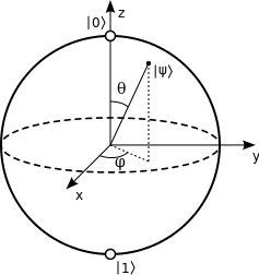
Another way to look at a qubit is in terms of the so called Bloch sphere, which gives us a nice way to visualize what is happening in quantum mechanical system that has two basis states. In the Bloch sphere picture, the qubit’s state \(\psi\) is a point on the surface of a unit sphere [1]:
Measurements on qubits
To obtain information from a quantum computer, one has to make a measurement of its’ qubits. As all other actions in a quantum computation, a measurement is also defined in terms of a set of operators. These measurement operators act on the state space of the system. Let’s take a look at the simplest case: measuring one qubit in the computational basis. As we learned when looking at the qubit, it has two computational basis states, say, \(\vert 0\rangle\) and \(\vert 1\rangle\). In principle one could choose arbitrary orthogonal states of the two-dimensional system to measure, but we use these for simplicity. There are two computational basis states in this case, so we get two possible measurement outcomes. The two measurement operators are then defined as follows:
\(M_0 = \vert 0\rangle\langle 0\vert\), with \(M_0^2 = M_0\)
\(M_1 = \vert 1\rangle\langle 1\vert\), with \(M_1^2 = M_1\)
The property of \(M_i^2 = M_i\) is important, because it ensures that the measurement operators fulfill the completeness relation: the sum of the probabilities for all measurement outcomes has to be one. The measurement operators are also Hermitian, which means that \(M_i = M_i^*\), so we get
\[I = M_0^\dagger M_0 + M_1^\dagger M_1 = M_0 + M_1\]Let’s look at the qubit again:
\[\vert \psi\rangle = \alpha \vert 0\rangle + \beta \vert 1\rangle\]When both \(\alpha\) and \(\beta\) are non-zero, the qubit is in a superposition state. Mathematically this is easy to formulate, but by the postulates of quantum mechanics, it turns out that we can only measure values of our system in a chosen basis - in the above example, these are the orthogonal states \(\vert 0\rangle\) and \(\vert 1\rangle\). Everything else in between can not be measured. In fact, as soon as a measurement is made, the superposition state collapses to one of the basis states, and the original amplitudes can not be recovered. As mentioned before, one can choose any pair of mutually orthogonal vectors of the qubit’s Hilbert space as a measurement basis. The choice of the measurement basis influences the outcome of the measurement. Let’s look at why this is the case by the example of a so called Pauli measurement, where we measure Pauli operators like \(X\), \(Y\) or \(Z\). The Pauli Z operator looks as follows:
\[Z = \begin{bmatrix} 1 & 0\\ 0 & -1 \\ \end{bmatrix}\]This has the eigenvectors \(\vert 0\rangle\) and \(\vert 1\rangle\), and eigenvalues \(\pm 1\). When applying this operator to a qubit, its’ value changes along the \(z\) axis in the Bloch sphere picture. A measurement gives us information about where the state approximately lies on the sphere. Namely, it divides the state space into two subspaces, and after measuring the qubit, we know probabilistically in which subspace the state was: when measuring \(\vert 0\rangle\), it was probably in the subspace of eigenvalue \(1\), when measuring \(\vert 1\rangle\), it was probably in the subspace of eigenvalue \(-1\). I write probably, because as we saw above, we measure states with probabilities given by their amplitudes, so unless one of the states has an amplitude of 0, it could always be our measurement outcome even though the amplitude for the other state is much higher. As we didn’t change anything in terms of the axes we use to describe the qubit, this is equivalent to making a measurement in the computational basis. Using another measurement basis for a qubit means choosing another way to divide the state space into two subspaces. This can be done by choosing any operator that has two unique eigenvalues, usually \(\pm 1\), like any of the other Pauli operators. For example, the Pauli X:
\[X = \begin{bmatrix} 0 & 1\\ 1 & 0 \\ \end{bmatrix}\]This is the quantum gate equivalent to the classical NOT gate, and rotates the state along the \(x\) axis. So when starting in the computational basis in state \(\vert 0\rangle\), the state is flipped to \(\vert 1\rangle\). When we now regard the \(x\) axis as our measurement basis, the state is on the equator of the Bloch sphere - yielding equal measurement probabilities for the states \(\vert 0\rangle\) and \(\vert 1\rangle\). This also means that measuring the \(X\) operator is equivalent to applying it on the state, followed by the \(H\) operator, and then measuring in the computational basis (along the \(z\) axis). To see why this is the case, let’s look at the \(H\) operator:
\[H = \frac{1}{\sqrt{2}} \begin{bmatrix} 1 & 1\\ 1 & -1 \\ \end{bmatrix}\]When applied on \(\vert 0\rangle\) or \(\vert 1\rangle\), the \(H\) operator creates the equal superposition of the two states - just what the \(X\) operator did when measuring in the \(X\) basis. Similarly, there exist operators for the other Paulis that transform the state into its equivalent along the \(z\) axis, so we can apply the corresponding operators and thereby “simulate” a measurement in another basis while still measuring along the \(z\) axis. By rotating the state according to the axis along which we want to measure, we can perform Pauli measurements even when the actual hardware only permits measurements in the computational basis.
What if our system has more than one qubit? It turns out that the above principles can easily be generalized to an arbitrary number of qubits. Let’s take the \(Z\) basis as an example and suppose we have a 4-qubit register \(\vert \psi\rangle = \vert 0001\rangle\). This state is a vector of length \(2^4 = 16\):
\[\vert \psi\rangle = \begin{pmatrix}1\\0\end{pmatrix} \otimes \begin{pmatrix}1\\0\end{pmatrix} \otimes \begin{pmatrix}1\\0\end{pmatrix} \otimes \begin{pmatrix}0\\1\end{pmatrix} = \begin{pmatrix}0 1 0 0 0 0 0 0 0 0 0 0 0 0 0 0 \end{pmatrix}^T\]Say we want to measure the second qubit in the \(Z\) basis. In the one-qubit case we would apply the \(Z\) operator to our state to calculate the measurement outcome. Now we will do the same in our multi-qubit system - but what do we do with the remaining qubits? If we only care about the measurement outcome of the second qubit and want to leave the others untouched, mathematically this is equivalent to applying the measurement operator on the second qubit and the identity on all others. So we create a measurement operator that looks as follows:
\[M_2 = I \otimes Z \otimes I \otimes I\]which yields a \(16 \times 16\) matrix, which we can now apply on the state \(\vert\psi\rangle\) to calculate the measurement outcome with regard to the second qubit. Notice that the \(Z\) operator is the second one in the product, because we want to measure with regard to the second qubit. If we want to also measure with regard to the third qubit, we add another \(Z\) instead of the \(I\) in the third place of the product, and so on.
This is called a projective measurement. It is described by an observable \(M\), like we just calculated above, which is a Hermitian operator on the state space of the system. We also saw that the measurement in the one-qubit case told us to which of the two eigenvalues of the system the measurement corresponds. In general, the observable \(M\) has a spectral decomposition
\[M = \sum_m mP_m\]where \(P_m\) is the projector onto the eigenspace of \(M\) with the corresponding eigenvalue \(m\). With these, we can calculate the probability \(p(m)\) of measuring in the eigenspace corresponding to \(m\) by
\[p(m) = \langle \psi\vert P_m \vert \psi \rangle\]In the above example we would calculate \(p(m) = \langle \psi\vert M_2 \vert \psi \rangle\). After the measurement, the state of the system is
\[\vert\psi_m\rangle = \frac{P_m \vert\psi\rangle}{\sqrt{p(m)}}\]It has been projected onto one of the basis vectors. Performing another measurement on \(\vert\psi_m\rangle\) using the same basis would mean projecting the projection of \(\vert\psi\rangle\) once more onto the same basis vector - so the measurement result is the same as before. A measurement is non-reversible, so once we have retrieved some information about the quantum system, we can never restore the original state vector.
Discussion and feedback